How close are we to predicting the structure of a protein from it's primary structure? Not very far! However,
prediction of secondary structure and regions of tertiary structure are quite good. These methods are mostly empirical and
are based on the actual structures of the 10,000 or so proteins whose structures are known. This large data base has been
examined to help determine rules which can be used to predict the disposition of a particular amino acid in a protein.
Secondary Structure
As we have seen previously, amino acids vary in their propensity to be found in alpha helices, beta strands,
or reverse turns (beta bends, beta turns). These difference can be rationalized from the structure of each amino
acid, as described before.
Figure: Amino Acid Structure and propensity for secondary structure
From the data bases, propensities can be calculated to determine the likelihood that a given amino acid
will be in one of those structures. Glycine for example would have a high propensity to be in reverse turns, while Pro, a
helix breaker, would have a low propensity to be in an alpha helix. A number is assigned to each amino acid
for each category of secondary structure. High numbers favor the likelihood that that amino acid would be in that structure.
The most popular list of propensities is from Chou-Fasman, where H indicates high propensity for secondary structure, h intermediate
propensity, i is inhibitory, b is a intermediate breaker, and B is a significant breaker of secondary structure.
Chou-Fasman Amino Acid Propensities
| A.A. |
Helix |
Sheet |
| Designation |
P |
Designation |
P |
| Ala |
H |
1.42 |
i |
0.83 |
| Cys |
i |
0.70 |
h |
1.19 |
| Asp |
I |
1.01 |
B |
0.54 |
| Glu |
H |
1.51 |
B |
0.37 |
| Phe |
h |
1.13 |
h |
1.38 |
| Gly |
B |
0.57 |
b |
0.75 |
| His |
I |
1.00 |
h |
0.87 |
| Ile |
h |
1.08 |
H |
1.60 |
| Lys |
h |
1.16 |
b |
0.74 |
| Leu |
H |
1.21 |
h |
1.30 |
| Met |
H |
1.45 |
h |
1.05 |
| Asn |
b |
0.67 |
b |
0.89 |
| Pro |
B |
0.57 |
B |
0.55 |
| Gln |
h |
1.11 |
h |
1.10 |
| Arg |
i |
0.98 |
i |
0.93 |
| Ser |
i |
0.77 |
b |
0.75 |
| Thr |
i |
0.83 |
h |
1.19 |
| Val |
h |
1.06 |
H |
1.70 |
| Trp |
h |
1.08 |
h |
1.37 |
| Tyr |
b |
0.69 |
H |
1.47 |
Next a stretch of amino acids about 7 amino acids is taken, starting from the N-terminal of the protein.
First the average alpha helical propensities for amino acids 1-7 are determined and assigned, let's say, to the middle (4th)
amino acid in that sequence. Then alpha helical propensities for amino acids 2-8 are averaged and assigned to the middle (5)
amino acid in that range. This continues until all but the first and last few amino acids have an average value assigned to
them. If a contiguous stretch of amino acids has high average propensity, they are probably in an alpha helix in the native
protein. This process is repeated using beta strand and reverse turn propensities. The final assignments of most probably
secondary structure are made. Of course this system was tested against proteins whose tertiary structure was known. See the
results for secondary structure prediction for one protein. In this example, the average propensity for four contiguous amino acids is calculated (starting with amino
acids 1-4, then amino acids 5-8, etc, and continuing to the end of the polypeptide). Next this process is repeated for
contiguous stretches 2-5, 6-9, etc, and continuing to the end.
Amphiphilic Helices
Additional information about putative helices can be obtained by determining if they are amphiphilic (one
side of the helix containing mostly hydrophobic side chains, with the opposite side containing polar or charged side chains.
A helical wheel projection can be made. In this a circle is draw representing a downward cross-sectional view of the helix
axis.
Figure: Helical wheel projection
The side chains are placed on the outside of the circle, staggered in a fashion determined by the fact
that there are 3.6 amino acids per turn of the helix. If one side of the wheel contains predominantly nonpolar side chains
while the other side has polar side chains, the helix is amphiphilic. Imagine how such helices might be packed in a protein.
Hydrophobic Structure
In a completely analogous fashion, a hydrophobic propensity or hydopathy can be calculated. In this system, empirical measures of the hydrophobic nature of the side chains are used to assign a number
to a given amino acid. Many hydropathy scales are used. Several are based on the Dmo
transfer of the side chains from water to a nonpolar solvent. Two commonly used scales are the Kyte-Doolittle Hydropathy and Hopp-Woods scales (used more like a hydrophilicity index to predict surface or water accessible structures that might be recognized
by the immune system)
Hydrophobicity Indices for Amino Acids
|
Amino Acid |
Kyte-Doolittle |
Hopp-Woods |
|
Alanine |
1.8 |
-0.5 |
|
Arginine |
-4.5 |
3.0 |
|
Asparagine |
-3.5 |
0.2 |
|
Aspartic acid |
-3.5 |
3.0 |
|
Cysteine |
2.5 |
-1.0 |
|
Glutamine |
-3.5 |
0.2 |
|
Glutamic acid |
-3.5 |
3.0 |
|
Glycine |
-0.4 |
0.0 |
|
Histidine |
-3.2 |
-0.5 |
|
Isoleucine |
4.5 |
-1.8 |
|
Leucine |
3.8 |
-1.8 |
|
Lysine |
-3.9 |
3.0 |
|
Methionine |
1.9 |
-1.3 |
|
Phenylalanine |
2.8 |
-2.5 |
|
Proline |
-1.6 |
0.0 |
|
Serine |
-0.8 |
0.3 |
|
Threonine |
-0.7 |
-0.4 |
|
Tryptophan |
-0.9 |
-3.4 |
|
Tyrosine |
-1.3 |
-2.3 |
|
Valine |
4.2 |
-1.5 |
For a water-soluble protein, a continuous stretch of amino acids found to have a high average hydropathy
is probably buried in the interior of the protein. Consider the example of bovine a-chymotrypsinogen, a 245 amino acid protein, whose sequence is shown below in single letter code.
1 CGVPAIQPVLSGLSRIVNGEEAVPGSWPWQVSLQDKTGFHFCGGSLINENWVVTAAHCGV
61 TTSDVVVAGEFDQGSSSEKIQKLKIAKVFKNSKYNSLTINNDITLLKLSTAASFSQTVSA
121
VCLPSASDDFAAGTTCVTTGWGLTRYTNANTPDRLQQASLPLLSNTNCKKYWGTKIKDAM
181 ICAGASGVSSCMGDSGGPLVCKKNGAWTLVGIVSWGSSTCSTSTPGVYARVTALVNWVQQ
241
TLAAN
A hydrophathy plot for chymotrypsinogen (sum of hydropathies of seven consecutive residues) shows many
stretches that are presumably buried in the interior of the protein.
Figure: hydrophathy plot for chymotrypsinogen
Membrane Proteins
So far we have discussed predominantly globular proteins that are soluble in water. Proteins are also found associated
with membranes. Two major classes of membrane proteins are found in nature.
- peripheral membrane proteins: water soluble proteins bound reversibly and non-covalently
to the membrane through electrostatic attractions between charged polar head groups of the phospholipids and the protein.
These proteins can often be released from the membrane by addition of high salt, since they are often attracted to the bilayer
by electrostatic interactions between charged phospholipid head groups and polar/charged groups on the protein surface.
- integral membrane proteins: actually insert into the bilayer. These can be released
from the membrane and effectively solubilized by the addition of single chain amphiphiles (detergents) which form a mixed
micelle with the integral membrane protein. Nonionic detergents (Trition X-100, octylglucoside, etc) are often used
in the purification of membrane proteins. Ionic detergents (like SDS) not only solubilize the integral membrane proteins,
but also denature them.
Figure: Types of membrane proteins
In some of these integral membrane proteins, large extracellullar and intracellular domains of the protein
are present, connected by the intramembrane regions. The intramembrane spanning region often consists of either a single alpha
helix, or 7 different helical regions which zig-zag through the membrane. These transmembrane sequences can readily
be determined through hydropathy calculations. For example, consider the integral membrane bovine protein rhodopsin.
Its 348 amino acid sequence (in single letter code) is shown below:
MNGTEGPNFYVPFSNKTGVVRSPFEAPQYYLAEPWQFSMLAAYMFLLIMLGFPINFLTLY
VTVQHKKLRTPLNYILLNLAVADLFMVFGGFTTTLYTSLHGYFVFGPTGCNLEGFFATLG
GEIALWSLVVLAIERYVVVCKPMSNFRFGENHAIMGVAFTWVMALACAAPPLVGWSRYIP
EGMQCSCGIDYYTPHEETNNESFVIYMFVVHFIIPLIVIFFCYGQLVFTVKEAAAQQQES
ATTQKAEKEVTRMVIIMVIAFLICWLPYAGVAFYIFTHQGSDFGPIFMTIPAFFAKTSAV
YNPVIYIMMNKQFRNCMVTTLCCGKNPLGDDEASTTVSKTETSQVAPA
Rhodopsin hydropathy plot calculations shows that is contains seven transmembrane helices which
wind through the membrane in a serpentine fashion..
Figure: Rhodopsin hydropathy plot
Figure: seven transmembrane helices
Rhodopsin Hydropathy Results
| No. |
N terminal |
transmembrane region |
C terminal |
type |
length |
| 1 |
40 |
LAAYMFLLIMLGFPINFLTLYVT |
62 |
PRIMARY |
23 |
| 2 |
71 |
PLNYILLNLAVADLFMVFGGFTT |
93 |
SECONDARY |
23 |
| 3 |
113 |
EGFFATLGGEIALWSLVVLAIER |
135 |
SECONDARY |
23 |
| 4 |
156 |
GVAFTWVMALACAAPPLVGWSRY |
178 |
SECONDARY |
23 |
| 5 |
207 |
MFVVHFIIPLIVIFFCYGQLVFT |
229 |
PRIMARY |
23 |
| 6 |
261 |
FLICWLPYAGVAFYIFTHQGSDF |
283 |
PRIMARY |
23 |
| 7 |
300 |
VYNPVIYIMMNKQFRNCMVTTLC |
322 |
SECONDARY |
23 |
Membrane proteins call be solubilized by addition of single chain amphiphiles (detergents).
The nonpolar tails of the detergents interact with the hydrophobic transmembrane domain of the membrane protein forming a
"mixed" micelle-like structure. Nonionic detergents like Triton X-100 and octyl-glucoside are often used to solubilize
membrane proteins in their near native state. In contrast, ionic detergents like sodium dedecyl sulfate (with a negatively
charged head group) denature proteins during the solubilization process. To study membrane proteins in a more native-like
environment, proteins solubilized by nonionic detergent can be reconstituted into bilayer liposome structures using methods
similar to those from Lab 1 in which you prepared dye-capsulated large unilamellar vesicles (LUVs). However, it can
be difficult to study the intra- and extracellular domains of membrane proteins in liposomes, given that one of those domains
is hidden inside the liposome. A novel technique that removes this barrier was recently developed by Sligar. He
created an amphiphilic protein disc with an opening in the center. The inner opening is lined with nonpolar residues,
while the outer surface of the disc is polar. When the discs were added to phosphlipids, small bilayers formed inside
the disc. Membrane proteins like the b-2 adrenergic receptor could
be reconstituted in the nanodisc bilayers, allowing solvent exposure of both the intracellular and extracellular domains of
the receptor protein.
Figure: Nanodisc with membrane protein
Protein Tertiary Structure
We are getting closer to predicting the tertiary structure of a protein, but as we have seen from molecular
mechanics and dynamics calculations, it is a huge computational task. There are two basic approaches which are often
combined.
- calculations using energy minimization and statistical mechanics: These "semi-empirical"
techniques don't assume any given secondary structure propensities or hydrophobicities. Such methods have produced limited
success with small proteins whose actual structure is known.
- homology modeling based on proteins of known structure: The structures of about
10,000 different proteins are known. This can serve as an empirical data base of possible conformations. Instead
of an infinite number of prototypical structures, it is becoming clear that there may be a reasonably low number (in the hundreds)
of basic structural motifs that are used over and over in nature. By aligning the amino acid sequences of
different proteins, and comparing their properties (such as secondary structure propensities, hydrophobicities, etc.), probable
low energy structures of the new protein can be determined. This initial structure can be run through multiple minimization
and dynamic simulations to produce a tentative "lowest" energy structure. The structure should be compact (checked through
calculation of packing density) and experimental techniques (such as spectroscopic methods) should be employed to validate
the structure.
Many models of the actual folding process have been presented, most of which have some experimental support.
In one, a hydrophobic collapse of the protein produces a seed structure upon which secondary structure and final tertiary
collapse results. Alternatively, initial formation of an alpha helix might serve as the seed structure. A combination
of the two is likely. In one scenario, two small amphiphilic helices might form which interact through their nonpolar
faces to produce the initial seed structure.
Many studies have been done on a domain of the protein villin. A company at Stanford University
(Folding at Home) actually allows you to process protein folding data on your own computer when you're not using it (an example of distributed
computing). The example below shows one simulation of length greater than 1 ms.
In the simulation, it collapses to a near native-like state then unfolds again as it iteratively probes conformational space
as it "seeks" the global energy minimum.
Zhou and Karplus recently simulated the folding of residues 10-55 of Staphylococcus aureus protein
A which form a 3-helix bundle structure.
Figure: 3-helix bundle
Using molecular dynamics, they carried out 100 folding simulations. Two types of folding trajectories
were noted.
- In the first type, helices form early (70% within 10 ns), but the fraction of native interhelical contacts
(indicating proper packing of the helices together) and the overall packing density are not similar to the native state.
Then the helices diffuse and collide with each (in the rate-limiting step) until the native state is reached at about 19 ms. In this model, non-obligatory intermediates can occur (due to collapse to non-native
interhelical packing in the rate-limiting step) which could slow down folding.
Figure: helices form early
- In another type, there is a simultaneous and quick partial helix formation and collapse (90% at 200 ns),
to a state which is similar to the molten globule. At this point, only about 20% of the native contacts are present.
The final tertiary structure is achieved after a slow process of forming native contacts within the compact state, which takes
about 500 ms.
Figure: simultaneous and quick partial helix formation and collapse
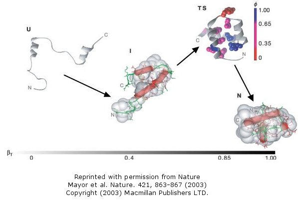
The Fersht lab has been combining experimental and theoretical approaches to the folding/unfolding of another three helix
bundle protein, Engrailed homeodomain.
Figure: Engrailed homeodomain
This protein is among the fastest folding and unfolding proteins known (ms time scale).
This time frame is also amenable to study through molecular dynamics simulations. Both sets of data support a folding
pathway in which the unfolded state (U) collapses in a microsecond to an intermediate state (I) characterized by significant
native secondary structure and mobile side chains that is less compact than the native state (N). The I state hence
resembles the molten globule state. To more clearly understand the unfolded state, they generated a mutant (Leu16Ala)
which was only marginally stable at room temperature (2.5 kcal/mol). Spectroscopic measurements (CD, NMR) showed this
state to resemble the intermediate (I) state, with much native secondary structure and a 33% greater radius of gyration than
the N state. In effect they could study the transient intermediate of the wild type protein more easily by making that
state more stable through mutagenesis. These studies showed that the intermediate is on the folding pathway and not
inhibitory to the process. Using molecular dynamic simulations, the intermediate to native state transition was shown
to proceed via a transition state (TS) in which the native secondary structure is almost all present and the helices are engaged
in the final packing process.
Figure: Complete Folding Pathway of Engrailed Homeodomain by Experiment and Simulation
The holy grail in protein folding research has always been to predict the tertiary structure of a protein given its primary
sequence. A similar but conceptually easier problem is to design a protein which will fold to a given structure with
predicted secondary structure. Many possible sequences could be designed to fold to the desired structure, which makes
this problem easier compared to the folding of a given sequence to just one native state. Kuhlman et al. have recently
accomplished such a feat for a synthetic protein of 93 amino acids which they designed to fold to a unique topology not yet
observed in nature. This represents a significant advance over earlier attempts in which mimics of known proteins were
made. Such structures would be expected to fold in analogous fashions to the parent protein because of the necessary
constraints placed by the need to fold to a compact state.
 Chime Model: Top7 - A designed 93 amino acid protein with a novel fold
 Online LIterature: