The following derivations and graphs are derived from the equation for fractional saturation Y = [L]/(Kd
+ [L]). Assume that the error in Y is +/- 0.02 at each [L] for the following analysis. Likewise, consider a constant error
in L
A. HYPERBOLIC PLOT: FIT TO NONLINEAR EQUATION.
For the equilibrium: M + L <==> ML, [ML] = ([Mo][L])/(Kd + [L])
or: fractional saturation = Y = [L]/(Kd + [L]).
A plot of Y vs gives a hyperbola, as shown in the figure below.
Figure: Hyperbola
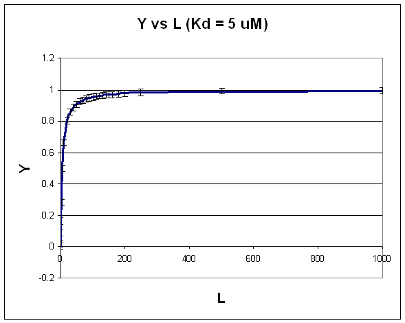
Note that the constant error bars are shown on the diagram as well. Remember, you can not easily determine
the Kd from a hyperbolic fit (Kd = L at half saturation) unless you have truly reached saturation. A better way to determine
Kd from hyperbolic binding data is to actually fit all the data to an equation for a hyperbola using a non-linear regression
program, such as found in Mathcad. Remember, however, bad data can still be fit.
 Mathcad 8 - Nonlinear Hyperbolic Fit. A: Mo and Kd | B: Kd
B. DOUBLE-RECIPROCAL PLOT: FIT TO LINEAR REGRESSION EQUATION.
1/Y = (Kd + L)/L = (Kd/L) + 1
This double-reciprocal plot is the form y = mx + b, where y = 1/Y, m = Kd, x = 1/L, and b = 1.
Figure: double-reciprocal plot
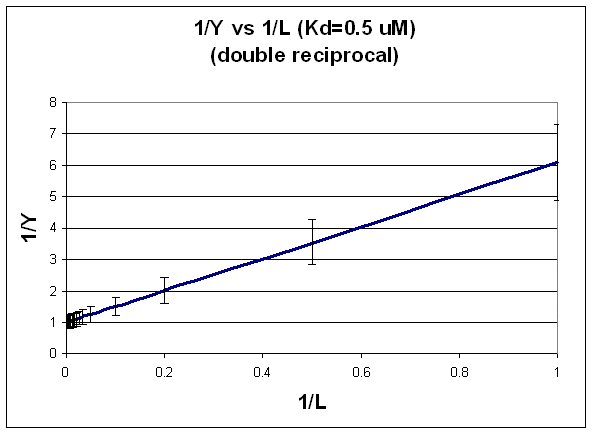
Notice in this that the errors are not constant. This is easily shown by the following example.
If Y = 1 +/- 0.02 (as in the above examples), then
Y could vary from 0.98 - 1.02 (range of 0.04). 1/Y
would vary from 1/1.02 - 1/0.98 or 0.98 - 1.02. (range of 0.04)
If, Y = 0.1 +/- 0.02, then Y could vary from 0.08 -0.12, a range again of 0.04. But now, 1/Y would vary
from 1/0.12 - 1/0.08, or 8.33 - 12.5, (range of 4.17! Notice that as Y is smaller, I/Y get bigger and the error "envelope"
gets larger.
You can not legitimately use linear regression analysis on the straight line double reciprocal plot, since
the error at each point is not constant. You can use LR analysis to determine the slope if you can weight each point differently.
Clearly in this case, the higher Y or lower 1/Y values would be weighted more. Given the availability of computer programs
for fitting non-linear equations, the linear double-reciprocal plot is not used often to extract the best value of Kd.
However, it is very useful in getting an estimate of Kd which can then be used in a non-linear fit as described in A.
In addition, it still has widespread use in the visual analysis of multiple binding curves in the absence and presence of
different concentrations of an inhibitor of binding. We will see this use later when we study enzyme kinetics.
C. SCATCHARD PLOT FIT TO LINEAR REG. EQUATION:
Y(Kd + L) = L OR Y Kd + YL = L or
Ykd = L - YL = L (1 - Y) which gives
Y/L = (1-Y)/Kd = -Y/Kd + 1/Kd
This equation, known as the Scatchard equation, is of the form y = mx + b, where
y = Y/L, x = Y, m = -1/Kd, and b = 1/Kd.
Figure: Scatchard Equation
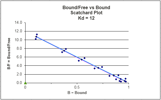
The same error envelop problems exist for this plot. In this plot, the error associated with the x axis
variable Y is constant. However, Y/L is plotted on the y axis so the error associated with this calculation is not constant.
This fitting method is one of the most misused.
Notice that Y/L appears to go to 0/0 when L approaches 0. This actual limiting
value can be determined from l'Hopital's rule: the limiting ratio is given by the limit of the derivative of the numerator
(Y) divided by the derivative of the denominator (L). This value is 1/Kd.
Curvilinear Scatchard plots are often observed. These can result from several reasons, including:
- a mixture of two different M's, with different Kd's
- M binding more than 1 ligands with different Kd's
- M binding more than 1 ligand in which binding of the first decreases the Kd for the second (positive
cooperativity) or vice-versa (negative cooperativity).
D. SEMI-LOG PLOT:
The best way to visualize whether saturation is reached is by plotting Y vs log L since the plot rises steeply and plateaus quickly compared to the hyperbolic plot which plateaus slowly.
Figure: Y vs log L
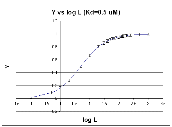
Second, it is logical to plot Y vs log L since the extent of binding is determined by the chemical potential
of L and M, and the chemical potential of L is proportional to log L. Even if you get a good non-linear fit to a hyperbola
(as in A above), you should do a Y vs log L plot to see how close to saturation you have come.
We can think about the nature of the Y vs log L plot by comparing it to the results we derived using the
Henderson-Hasselbach equation. From that equation, we could calculate, given a pH, the protonation state of an
acid. We determined that if the pH was 2 units below the pKa, the ratio of [HA]/[A-] = 100/1 or about 100% of the acid
was protonated. Likewise, if the pH was 2 units above the pKa, the ratio of [HA]/[A-] = 1/100 or about 100% of the acid
was deprotonated. If the pH = pKa, 50% of the acid was protonated. In this example we really looked at
fractional saturation of the acid (i.e. how much was bound to protons) as a function of the log L where L was [H3O+].
Now lets apply this to the equilibrium M + L <==> ML. We wish to know how much is bound, or
the fractional saturation, as a function of the log L. Consider three examples.
- L = 0.01 Kd (i.e. L << Kd), which implies that Kd = 100L. Then Y = L/[Kd+L] = L/[100L + L]
≈1/100. This implies that irrespective of the actual [L], if L = 0.1 Kd, then Y ≈0.01.
- L = 100 Kd (i.e. L >> Kd), which implies that Kd = L/100. Then Y = L/[Kd+L] = L/[(L/100)
+ L] = 100L/101L ≈ 1. This implies that irrespective of the actual [L], if L = 100 Kd,
then Y ≈1.
- L = Kd, then Y = 0.5
These scenarios show that if L varies over 4 orders of magnitude (0.01Kd < Kd < 100Kd),
or, in log terms, from
-2 + log Kd < log Kd < 2 + log Kd), irrespective of the magnitude
of the Kd, that Y varies from approximately 0 - 1. In other words, Y varies from 0-1 when L varies from log Kd by +2.
Hence, plots of Y vs log L for a series of binding reactions of increasingly higher Kd would reveal a series of identical
sigmoidal curves shifted progressively to the right.
NOTE: I have derived equations and plots above using the variables Y and L. Remember, Y = ML/Mo. I could
easily substitute ML/Mo is all of the above equations, and get plots using ML and L. Mo, a constant, would then be factored
into the slope and intercept terms.